Xpansion settings¶

Optimization¶

UC type¶

enum The unit-commitment type parameter specifies the simulation mode used by Antares to evaluate the operating costs of the electrical system:

expansion_fast: Deactivate the flexibility constraints of the thermal units (Pmin constraints and minimum up and down times), and don't take into account either the start-up costs or the impact of the day-ahead reserve.
expansion_accurate: The unit-commitment variables are relaxed. The flexibility constraints of the thermal units as well as the start-up costs are taken into account.

Master problem¶

int The master parameter provides information on how integer variables are taken into account in the Antares Xpansion master problem.

relaxed: The integer variables are relaxed, and the level constraints of the investment candidates (cf. unit-size) will not be necessarily respected. The master problem is linear.
integer: The investment problem is solved by taking into account unit-size constraints of the candidates. The master problem is a MILP (Mixed-Integer Linear Program).

For problems with several investment candidates with large max-units, using master = relaxed can accelerate the Antares-Xpansion algorithm very significantly.

Max iteration count¶

int Maximum number of iterations for the Benders decomposition algorithm. Once this number of iterations is reached, the Antares Xpansion algorithm ends, regardless of the quality of the solution.

Absolute optimality gap (€)¶

float The optimality gap defined in euros, is the tolerance for the Antares Xpansion algorithm.

At each iteration, the algorithm computes upper and lower bounds on the optimal cost. The algorithm stops as soon as the quantity best_upper_bound - best_lower_bound falls below optimality_gap. The solution returned by the algorithm has a cost equal to best_upper_bound, which is guaranteed to be within optimality_gap euros of the optimal cost.

If optimality_gap = 0, Antares-Xpansion will continue its search until the optimal solution of the investment problem is found.
If optimality_gap > 0, the search will stop as soon as best_upper_bound - best_lower_bound < optimality_gap.

Here is an illustration of the optimality gap and the set of solutions that can be returned by the package when the gap is strictly positive.

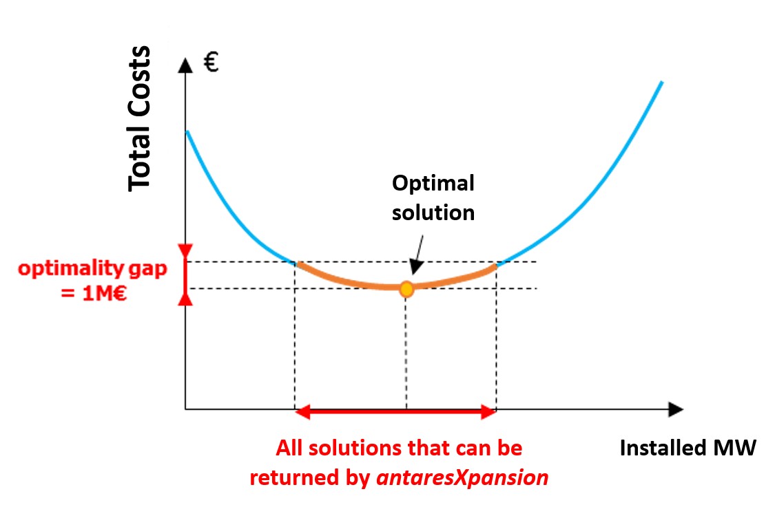
The interest of a strictly positive optimality_gap is that it speeds up the search by stopping as soon as a "good" solution is found.

The interpretation of this stopping criterion is not always obvious. It certainly guarantees that a solution found by the algorithm has a cost that is close to the optimum, but it does not provide any information on the distance (in MW) between the installed capacities of this solution and those of the optimal solution: if the cost function is relatively flat around the optimum, solutions whose costs are close may have significantly different installed capacities (see Figure 10).

Which settings should I use for the optimality_gap?

I have to run several expansion optimizations of different variants of a study and compare them. In that case, if the optimal solutions are not returned by the package, the comparison of several variants can be tricky. The inaccuracy of the method might indeed be of the same order of magnitude as the changes brought by the input variations. It is therefore advised to be as closed as possible from the optimum of the expansion problem. To do so, we advise to set the optimality_gap to zero.
I am building one consistent generation/transmission scenario. As the optimal solution is not more realistic than an approximate solution of the modelled expansion problem, the settings can be less constraining with an optimality_gap of a few million euros.

Relative optimality gap¶

float Tolerance on the relative gap for the Antares Xpansion algorithm.

At each iteration, the algorithm computes upper and lower bounds on the optimal cost. The algorithm stops as soon as the quantity (best_upper_bound - best_lower_bound) / max(|best_upper_bound|, |best_lower_bound|) falls below relative_gap. For a relative gap \(\alpha\), the cost of the solution returned by the algorithm satisfies:

\[\frac{{\scriptstyle\texttt{xpansion solution cost}} - {\scriptstyle\texttt{optimal cost}}}{{\scriptstyle\texttt{optimal cost}}} < \alpha .\]

Note

The algorithm stops as soon as the first criterion among optimality_gap and relative_gap is met. Keep in mind that if either parameter is not specified by the user, the default value is used.

Relaxed optimality gap¶

float The relaxed_optimality_gap parameter only has effect when master = integer. In this case, the master problem is relaxed in the first iterations. The relaxed_optimality_gap is the threshold from which to switch back from the relaxed to the integer master formulation.

In the first iterations, the algorithm computes upper and lower bounds on the optimal cost of the relaxed master problem. The algorithm switches to the integer formulation as soon as the quantity (best_upper_bound - best_lower_bound) / best_upper_bound falls below relaxed_optimality_gap. For the subsequent iterations, the best upper bound is reset to \(+\infty\) as the solutions of the relaxed problem are not feasible for the integer formulation.

Solver¶

enum Solver that is used to solve the master and the subproblems in the benders decomposition. The user can set Cbc which stands for the COIN-OR optimization suite. Depending on whether the problem has integer variables, Antares Xpansion calls either the linear solver (Clp) or the MILP solver (Cbc) of the COIN-OR optimization suite.

Note

In Antares Xpansion, the subproblems are always linear. If master = relaxed, the master problem is linear as well, whereas if master = integer, the master problem is a MILP.

Separation parameter¶

float Defines the step size for the in-out separation in \([0,1]\). If \(x_{in}\) is the current best feasible solution and \(x_{out}\) is the master solution at the current iteration, the investment in the subproblems is set to

\[ x_{cut} = {\small \texttt{separation parameter}} * x_{out} + (1 - {\small \texttt{separation parameter}}) * x_{in} .\]

The in-out stabilisation technique is used in order to speed up the Benders decomposition. When separation_parameter < 1, it is necessary to relax the master problem in the first iterations as the cut point \(x_{cut}\) is a convex combination of the best feasible solution and of the solution of the master problem. In the case where master = integer, the algorithm proceeds as follows:

Solve the first iterations with the relaxed formulation using the in-out stabilisation technique
Once the gap is sufficiently small (see relaxed_optimality_gap), switch back to the integer formulation and set back separation_parameter = 1 i.e. use the classical Benders algorithm.

Time limit (h)¶

int Maximum allowed time in seconds for the execution of the Benders step of Antares Xpansion (i.e. the time of the initial Antares simulation and for the problem generation step is not accounted for). Once the timelimit is reached, the algorithm finishes the current Benders iteration - which can take several additional seconds or minutes - and terminates.

Batch size¶

int This parameter specifies the number of subproblems per batch. If set to 0, then all subproblems are in the same batch. In this case, the classical Benders is launched.

Log level¶

enum Possible values: {0, 1, 2}, specifying the solver's log severity. Default value: 0.

Logs can be printed both in the console and in a file. There are 3 types of logs:

Operational: Displays progress information for the investment on candidates and costs,
Benders: Displays information on the progress of the Benders algorithm,
Solver: Logs of the solver called for the resolution of each master or subproblem.

The table below details the behavior depending on the log_level.

	Operational	Benders	Solver
File	Always `(reportbenders.txt)`	Always `(benders_solver.log)`	2 `(solver_log_proc_<proc_num>.txt)`
Console	0	>= 1	Never

Cut coefficient tolerance¶

float Tolerance under which cuts coefficients and right-hand sides are considered to be zero. This allows to have "clean" cuts in the master problem, in order to avoid numerical issues. This should be less than 1.

Master solution tolerance¶

float Control the tolerance used when rounding the solution variables of the master problem. It allows to restore feasibilities of master solutions (as the solver may return slightly infeasible values). Also in the stabilized version (i.e. when separation_parameter < 1), if x_cut is within this tolerance of a bound, it will be rounded to this bound before fixing the subproblems candidates values. This helps to avoid numerical artifacts.

Modeling add-ons¶

Yearly weight¶

string The parameter yearly-weights allows to assume that the Monte Carlo years simulated in the Antares study are not equally probable. The most representative years may be given greater weight than those that are less representative. The yearly-weights parameter defines a file that stores a vector \(\left( \omega_{1},\ldots,\omega_{n} \right)\), with \(n\) the number of Monte-Carlo years in the study, which is used to evaluate the expected production cost:

\[ \mathbb{E}\left(\text{cost}\right) = \frac{\sum_{i = 1}^{n}{\omega_i\text{cost}_i}}{\sum_{i = 1}^{n}\omega_{i}} \ , \]

with \(\text{cost}_{i}\) the production cost of the \(i\)-th Monte Carlo jaar and \(\omega_i\) the associated weigth.

The input file must contain a single column with as many numerical values as there are Monte-Carlo years in the Antares study. The value of the \(i\)-th row is the weight \(\omega_i\) of the \(i\)-th Monte Carlo year.

Note

You can import the weights file in the Xpansion > Weights tab.

If the yearly-weights parameter is not used, the Monte-Carlo years of the Antares study are considered to be equally-weighted.

Note

The yearly-weights parameter must be set in line with the Antares study playlist by the user: years with zero weights must be removed from the Antares study playlist in order not to be simulated unnecessarily.

Additional constraints¶

string Name of the additional constraint file. It allows to impose linear constraints between the invested capacities of investment candidates. These linear constraints will be added to the master problem.

Note

You can import it in the Xpansion > Constraints tab.

The format of the file is inspired from binding constraints.

[1]                     # index
name = additional_c2    # Constraint name, unique and without any special symbols or space
semibase = 3            # Numeric coefficient of the variables
peak = 2                # Numeric coefficient of the variables
sign = less_or_equal    # Sign is less_or_equal, equal, or greater_or_equal
rhs = 300               # rhs is numeric and is the second term of the constraint

Here, the corresponding constraint equation is: \(3 \times \texttt{semibase} + 2 \times \texttt{peak} \leq 300\).

A constraint in the additional-constraints is defined with the following parameters:

name: string. The constraint name must be unique and must not contain any special symbols or space.
<investment-candidate-name>: float. Coefficient of the left-hand side variable corresponding to <investment-candidate-name>.
sign: Either less_or_equal, equal or greater_or_equal. Defines the relationship between the left-hand side and right-hand side of the constraint.
rhs: float. Right-hand side of the constraint.

The user can also optionally use binary constraints to represent, for example, exclusion constraints. The [variable] section is optional and allows the definition of optional variables linked to investment candidates for exclusion constraints.

Warning

The use of binary variables is not recommended as it greatly increases the calculation time.

Antares Xpansion cannot invest in semibase and peak at the same time, but it can invest in neither:

additional-constraint.ini

[variables]
semibase = bin_semibase
peak = bin_peak        
pv = bin_pv            

[1]
name = additional_c1
bin_semibase = 1        
bin_peak = 1            
sign = less_or_equal
rhs = 1

[2]
name = additional_c2
semibase = 3
peak = 2
sign = less_or_equal
rhs = 300

The above constraints translate to:

\(1 \times \texttt{bin_semibase} + 1 \times \texttt{bin_peak} \leq 1\)
\(3 \times \texttt{semibase} + \texttt{peak} \leq 300\)

Sensitivity calculation¶

Max gap to optimum (€)¶

float Defines the maximum gap with the optimal solution that is allowed.

Compute CAPEX¶

bool Whether to solve CAPEX sensitivity problems (minimization and maximization).

Projections¶

string List of candidate names for which the projection of the set of \(\varepsilon\)-optimal solutions is computed. For each candidate, two problems are solved: minimization and maximization of the invested capacity.