Advanced parameters

Seeds for random number

Defining random seeds allow to control random number generation for time series generation, noise (used to eliminate equivalent solution during the optimization) or reservoir levels.

Initial reservoir levels

enum DEPRECATED since 9.2 The reservoir level is now always determined with cold start behavior. Simulations results may in some circumstances be heavily impacted by this setting, hence proper attention should be paid to its meaning before considering changing the default value.

• cold start
• hot start

Cold vs. hot start

This parameter is meant to define the initial reservoir levels that should be used, in each system area, when processing data related to the hydropower storage resources to consider in each specific Monte-Carlo year.

As a consequence, Areas which fall in either of the two following categories are not impacted by the value of the parameter:

• No hydro-storage capability installed
• Hydro-storage capability installed, but the "reservoir management" option is set to false.

Areas that have some hydro-storage capability installed and for which explicit reservoir management is required are concerned by the parameter. The developments that follow concern only this category of Areas.

Cold Start

On starting the simulation of a new Monte-Carlo year, the reservoir level to consider in each Area on the first day of the initialization month is randomly drawn between the extreme levels defined for the area on that day.

• The value is drawn according to the probability distribution function of a "Beta" random variable, whose four internal parameters are set so as to adopt the following behavior:

  • Lower bound: Minimum reservoir level.
  • Upper bound: Maximum reservoir level
  • Expectation: Average reservoir level
  • Standard Deviation: (1/3) (Upper bound-Lower bound)

• The random number generator used for that purpose works with a dedicated seed that ensures that results can be reproduced from one run to another, regardless of the simulation runtime mode (sequential or parallel) and regardless of the number of Monte-Carlo years to be simulated.

Hot Start

On starting the simulation of a new Monte-Carlo year, the reservoir level to consider in each Area on the first day of the initialization month is set to the value reached at the end of the previous simulated year, if three conditions are met:

The simulation calendar is defined throughout the whole year, and the simulation starts on the day chosen for initializing the reservoir levels of all Areas.

The Monte-Carlo year considered is not the first to simulate, or does not belong to the first batch of years to be simulated in parallel. In sequential runtime mode, that means that year #N may start with the level reached at the end of year \(N-1\). In parallel runtime mode, if the simulation is carried out with batches of B years over as many CPU cores, years of the \(k\)-th batch 3 may start with the ending levels of the years processed in the \((k-1)\)-th batch.

The parallelization context must be set to ensure that the \(M\) Monte-Carlo years to simulate will be processed in a round number of \(K\) consecutive batches of \(B\) years in parallel

The first year of the simulation, and more generally years belonging to the first simulation batch in parallel mode, are initialized as they would be in the cold start option.

Note

Depending on the hydro management options used, the amount of hydro-storage energy generated throughout the year may either match closely the overall amount of natural inflows of the same year, or differ to a lesser or greater extent. In the case of a close match, the ending reservoir level will be similar to the starting level. If the energy generated exceeds the inflows (either natural or pumped), the ending level will be lower than the starting level (and conversely, be higher if generation does not reach the inflow credit). Using the hot start option allows to take this phenomenon into account in a very realistic fashion, since the consequences of hydro decisions taken at any time have a decisive influence on the system's long term future.

When using the reservoir level hot start option, comparisons between different simulations make sense only if they rely on the exact same options, i.e. either sequential mode or parallel mode over the same number of CPU cores.

More generally, it has to be pointed out that the "hydro-storage" model implemented in Antares can be used to model "storable" resources quite different from actual hydro reserves: batteries, gas subterraneous stocks, etc.

Use accuracy mode

enum

• wind
• solar
• load

Hydro heuristic policy

enum Define how the reservoir level should be managed throughout the year, either with emphasis put on the respect of rule curves or on the maximization of the use of natural inflows.

• accommodate rule curves Upper and lower rule curves are accommodated in both monthly and daily heuristic stages (described page 58). In the second stage, violations of the lower rule curve are avoided as much as possible (penalty cost on \(\Psi\) higher than penalty cost on \(Y\)). This policy may result in a restriction of the overall yearly energy generated from the natural inflows.
• maximize generation Upper and lower rule curves are accommodated in both monthly and daily heuristic stages (described page 58). In the second stage, incomplete use of natural inflows is avoided as much as possible (penalty cost on \(Y\) higher than penalty cost on \(\Psi\)). This policy may result in violations of the lower rule curve.

Hydro pricing mode

enum Define how the reservoir level difference between the beginning and the end of an optimization week should be reflected in the hydro economic signal (water values) used in the computation of optimal hourly generated or pumped power during this week.

• fast The water value is taken to remain about the same throughout the week, and a constant value equal to that found at the date and for the level at which the week begins is used in the course of the optimization. A value interpolated from the reference table for the exact level reached at each time step within the week is used ex-post in the assessment of the output variable "H.COST" (positive for generation, negative for pumping). This option should be reserved to simulations in which computation resources are an issue or to simulations in which level-dependent water value variations throughout a week are known to be small.
• accurate The water value is considered as variable throughout the week. As a consequence, a different cost is used for each increment of stock from/to which energy can be withdrawn/injected, in an internal hydro merit-order involving the 100 tabulated water-values found at the date at which the week ends. A value interpolated from the reference table for the exact level reached at each time step within the week is used ex-post in the assessment of the variable "H.COST" (positive for generation, negative for pumping). This option should be used if computation resources are not an issue and if level-dependent water value variations throughout a week must be accounted for.

Note

Simulations carried out in accurate mode yield results that are theoretically optimal as far as the techno-economic modelling of hydro (or equivalent) energy reserves is concerned. It may, however, require noticeably longer computation time than the simpler fast mode.

Simulations carried out in fast mode are less demanding in computer resources. From a qualitative standpoint, they are expected to lead to somewhat more intensive (less cautious) use of stored energy.

Power fluctuations

enum - free modulations - minimize excursions - minimize ramping

Shedding policy

enum Power shedding policy.

• shave peaks
• minimize duration

Day ahead reserve management

enum For the moment only one possibility global.

Unit commitment mode

enum Define the mode in which Antares solves the unit-commitment problem.

• fast Heuristic in which 2 LP problems are solved. No explicit modelling for the number of ON/OFF units.
• accurate Heuristic in which 2 LP problems are solved. Explicit modelling for the number of ON/OFF units. Slower than fast.
• MILP A single MILP problem is solved, with explicit modelling for the number of ON/OFF units. Slower than accurate.

Steps	Accurate	Fast
First optimization	Minimization of the overall system cost throughout the week in a continuous relaxed linear optimization. Fixed cost, Start-up cost, Pmin, Minimum Up/Down time are considered	Minimization of the overall system cost throughout the week in a continuous relaxed linear optimization. Fixed cost, Start-up cost, Pmin, Minimum Up/Down time are not considered
Heuristic	Calculate a unit-commitment compatible with the integrity constraints in the immediate neighborhood of the relaxed solution obtained in the first optimization.	Calculate a unit-commitment compatible with the first optimization, with the additional conditions: On- and Off- periods should be exact multiple of the higher of the two thresholds and Pmin should be respected
Second optimization	Take into account the integer variables found in the heuristic and solve again the optimal schedule problem for the week.	Take into account the integer variables found in the heuristic and solve again the optimal schedule problem for the week. Start-up costs as well as fixed costs are added ex post, but they are not considered to determine which units are on/off.

More on unit-commitment mode

Simulations carried out in accurate mode yield results that are expected to be close to the theoretical optimum as far as the techno-economic modelling of thermal units is concerned. They may, however, require much longer computation time than the simpler fast mode.

Simulations carried out in fast mode are less demanding in computer resources. From a qualitative standpoint, they are expected to lead to a more costly use of thermal energy. This potential bias is partly due to the fact that in this mode, start-up costs do not participate as such to the optimization process but are simply added ex post.

The weekly optimization problem belongs to the MILP (Mixed Integer Linear Program) class. The integer variables reflect, for each time step, the operational status (running or not) of each thermal unit. Besides, the amount of power generated from each unit can be described as a so-called semi-continuous variable (its value is either 0 or some point within the interval [Pmin , Pmax]). Finally, the periods during which each unit is either generating or not cannot be shorter than minimal (on- and off-) thresholds depending on its technology.

The unit-commitment mode parameter defines two different ways to address the issue of the mathematical resolution of this problem. In both cases, two successive so-called "relaxed" LP global optimizations are carried out. In-between those two LPs, a number of local IP (unit commitment of each thermal cluster) are carried out.

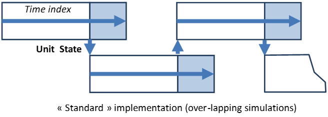
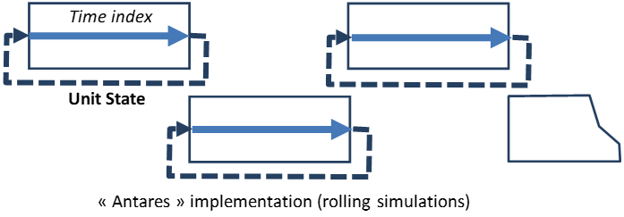
Besides, dynamic thermal constraints (minimum on- and off- time durations) are formulated on time-indices rolling over the week; this simplification brings the ability to run a simulation over a short period of time, such as one single week extracted from a whole year, while avoiding the downside (data management complexity, increased runtime) of a standard implementation based on longer simulations tiled over each other (illustration below).

Fast

In the first optimization stage, integrity constraints are removed from the problem and replaced by simpler continuous constraints.

For each thermal cluster, the intermediate IP looks simply for an efficient unit-commitment compatible with the operational status obtained in the first stage, with the additional condition (more stringent than what is actually required) that on- and off- periods should be exact multiple of the higher of the two thresholds specified in the dataset.

In the second optimization stage, the unit commitment set by the intermediate IPs is considered as a context to use in a new comprehensive optimal hydro-thermal schedule assessment. The amount of day-ahead (spinning) reserve, if any, is added to the demand considered in the first stage and subtracted in the second stage. Start-up costs as well as No-Load Heat costs are assessed in accordance with the unit-commitment determined in the first stage and are added ex post.

Accurate

In the first optimization stage, integrity constraints are properly relaxed. Integer variables describing the start-up process of each unit are given relevant start-up costs, and variables attached to running units are given No-Load Heat costs (if any), regardless of their generation output level. Fuel costs / Market bids are attached to variables representing the generation output levels.

For each thermal cluster, the intermediate IP looks for a unit-commitment compatible with the integrity constraints in the immediate neighborhood of the relaxed solution obtained in the first stage. In this process, the dynamic thresholds (min on-time, min off-time) are set to their exact values, without any additional constraint.

In the second optimization stage, the unit commitment set by the intermediate IP is considered as a context to use in a new comprehensive optimal hydro-thermal schedule assessment. The amount of day-ahead (spinning) reserve, if any, is added to the demand considered in the first stage and subtracted in the second stage.

Simulation cores

enum Allow to configure multi-threading.

• minimum
• low
• medium
• high
• maximum

Multi-threading in Antares

Multi-threading is also available on the proper calculation side, on a user-defined basis.

Provided that hardware resources are large enough, this mode may reduce significantly the overall runtime of heavy simulations.

To benefit from multi-threading, the simulation must be run in the following context:

• The parallel option must be enabled (it is disabled by default)
• The simulation mode must be either Adequacy or Economy

When the "parallel" solver option is used, each Monte-Carlo year is dispatched in an individual process on the available CPU cores. The number of such individual processes depends on the characteristics of the local hardware and on the value given to the study-dependent number of cores advanced parameter.

This parameter can take five different values (Minimum, Low, Medium, High, Maximum). The number of independent processes resulting from the combination (local hardware + study settings) is given in the following table, which shows the CPU allowances granted in the different configurations.

Starting from 9.2

Available CPU Cores	Minimum	Low	Medium	High	Maximum
1	1	1	1	1	1
2	1	1	1	2	2
3	1	1	2	3	3
4	1	1	2	3	4
5	1	2	3	4	5
6	1	2	3	5	6
7	1	2	4	6	7
8	1	2	4	6	8
9	1	3	5	7	9
10	1	3	5	8	10
11	1	3	6	8	11
12	1	3	6	9	12
S > 12	1	Ceil(S/4)	Ceil(S/2)	Ceil(3S/4)	S

Before 9.2

Available CPU Cores	Minimum	Low	Medium	High	Maximum
1	1	1	1	1	1
2	1	1	1	2	2
3	1